Hierarchical Cluster Analysis of USA states based on their Revenue and Expenditure, combined and separate, of 2013 data
In [34]:
library(dplyr)
library(ggplot2)
Data Source:
In [9]:
Finances2013=read.csv("SGF_2013_SGF003_with_ann.csv",
                       header=TRUE,stringsAsFactors=FALSE)
Finances2013=Finances2013 %>% select(GEO.display.label,SGF004,SGF005
                                     ,SGF007,SGF008,SGF009,SGF010,
                                     SGF011,SGF012,SGF013,SGF014,SGF036,SGF037,SGF038,SGF039,
                                     SGF040,SGF041,SGF042,SGF043,SGF044,SGF045,SGF046)
colnamess=paste0(Finances2013[1,],sep=",")
colnames(Finances2013)=colnamess
names(Finances2013)[names(Finances2013)=="Geographic area name,"] = "state"
Hierarchical Cluster Analysis of states based on their Expenditure and Revenue
In [10]:
colnames(Finances2013)
In [12]:
#Just cleaning data and changing char to numeric
Finances=Finances2013[-c(1,2),]
Finances[,c(2:22)]=sapply(Finances[,c(2:22)], as.numeric)
In [18]:
Built in function for Hierarchical Clustering in R
In [15]:
financesHClust=hclust(dist(Finances[,-1],method="euclidean"))
ExpRevgroups5 = cutree(financesHClust,5)
In [16]:
# draw dendogram
plot(financesHClust,labels=Finances[,1],hang = -1,cex = 0.6,
     main='State clusters based on their Revenue and Expenditure',xlab="States",ylab="distance")
rect.hclust(financesHClust, k=5, border=1:5)#"red")

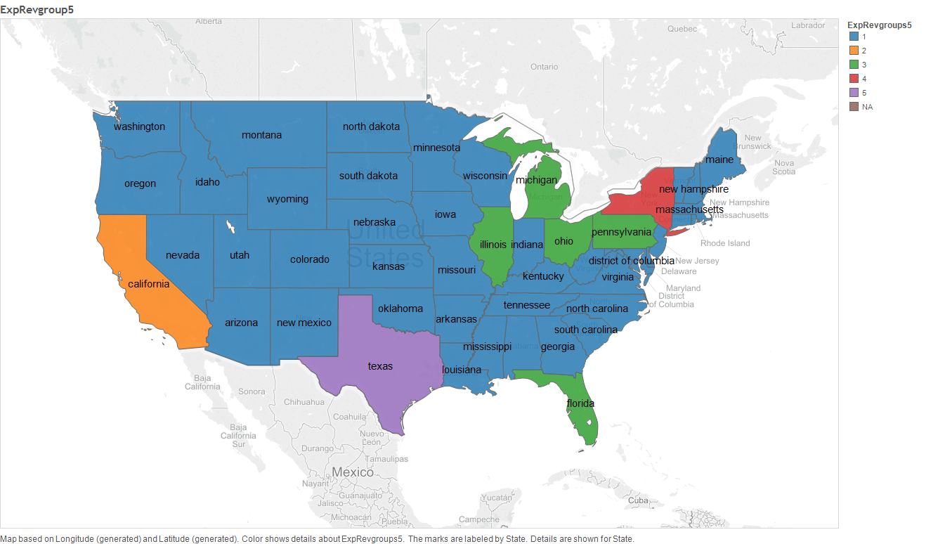
As we can see in the dendrogram, its clear that according to the Expenditure and Revenue values, 5 cluster is a logical cluster size. These clusters are;
- Cluster 1: Texas State
- Cluster 2: New York State
- Cluster 3: California State
- Cluster 4: Pennsylvania, Illinois, Ohio, Michigan and Florida
- Cluster 5: All states not listed above
In [17]:
Hierarchical Cluster Analysis based on State's Revenue Only
In [19]:
Finances2013Revenue=select(Finances,contains("Revenue")) # filtering columns which contain "Revenue"
Finances2013Revenue=cbind.data.frame(state=Finances[,1],Finances2013Revenue)
Stream of Revenues that are considered for the study are listed below. Note that, majority are revenues through tax.
In [20]:
colnames(Finances2013Revenue)
In [21]:
RevenueHClust=hclust(dist(Finances2013Revenue[,-1],method="euclidean"))
Revenuegroup5 = cutree(RevenueHClust,5)
plot(RevenueHClust,labels=Finances2013Revenue[,1],hang = -1,cex = 0.6,
     main='States cluster based on their 2013 Revenue Only ',xlab="States",ylab="distance")
rect.hclust(RevenueHClust, k=5, border=1:5)

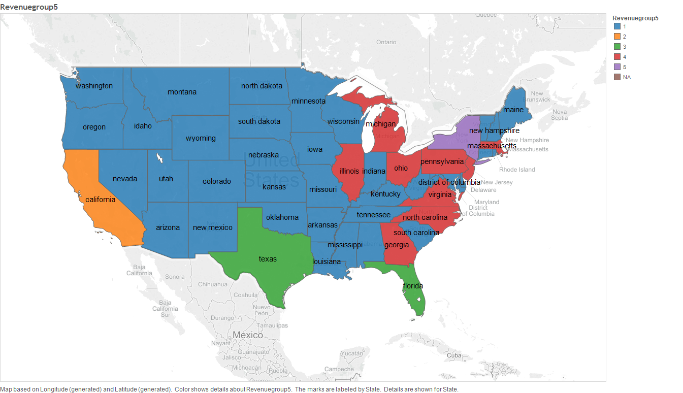
As we can see in the above dendrogram, its clear that, according to state's Revenue, cluster of size 5 is a significant size. The clusters under this clustering are:
- Cluster 1: California State
- Cluster 2: New York State
- Cluster 3: Texas State and Florida
- Cluster 4: Virginia, Georgia, North Carolina, Massachusetts, New Jersey,Illinois,Ohio, Michigan and Pennsylvania states
- Cluster 5: All states not clustered above
Hierarchical Cluster Analysis based on their Expenditure Only
In [22]:
Finances2013Exp=select(Finances,contains("Expenditure"))
Finances2013Exp=cbind.data.frame(state=Finances[,1],Finances2013Exp)
The functions of Expenditure are
In [24]:
colnames(Finances2013Exp)
In [25]:
ExpenditureHClust=hclust(dist(Finances2013Exp[,-1],method="euclidean"))
Expgroup5 = cutree(ExpenditureHClust,5)
plot(ExpenditureHClust,labels=Finances2013Exp[,1],hang = -1,cex = 0.6,
     main='States cluster based on their Expenditure amount Only',xlab="States",ylab="distance")
rect.hclust(ExpenditureHClust, k=5, border=1:5)

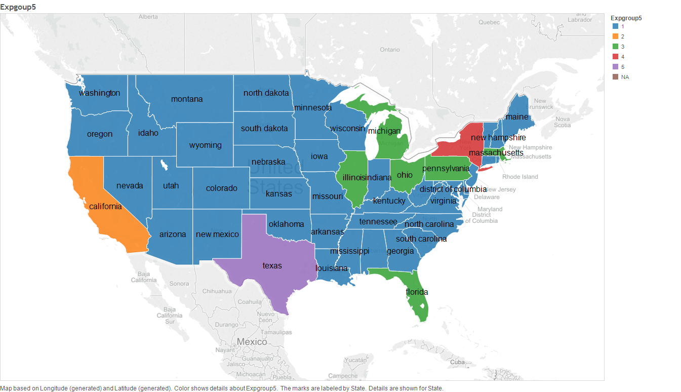
As we can see in the above dendrogram, its clear that the states clustered in to 5. These clusters are:
- Cluster 1: Texas State
- Cluster 2: New York State
- Cluster 3: California State
- Cluster 4: Illinois,Massachusetts, Florida,Pennsylvania,Michigan and Ohio States.
- Cluster 5: All states not clustered above
Summary
In [42]:
ByExpenditureAmount=c("California State","New York State","Texas State","Illinois, Massachusetts,
Florida, Pennsylvania, Michigan and Ohio States", "Others" )

ByRevenueAmount=c( "California State", "New York State", "Texas State and Florida"," Virginia, Georgia, North Carolina, Massachusetts, New Jersey,Illinois,Ohio, Michigan and Pennsylvania states", "Others")

ByRevenueExpenditureAmount=c("California State", "New York State","Texas State", "Pennsylvania, Illinois,Ohio, Michigan and Florida" , "Others")

summary=data.frame(ByExpenditureAmount,ByRevenueAmount,ByRevenueExpenditureAmount) rownames(summary)=c("Cluster_1", "Cluster_2", "Cluster_3", "Cluster_4", "Cluster_5")
summary